How to use GWAS atlas website
Contents
1. Browse GWAS summary statistics
2. Compare multiple GWAS
4. Frequently asked questions
2. Compare multiple GWAS
2.1. Select GWAS to compare
2.2. Summary of results
2.3. Pair-wise genetic correlation
2.4. Overlap of significant genes based on MAGMA gene analyses
2.5. Risk locus and gene pleiotropy
3. Create PheWAS plot2.2. Summary of results
2.3. Pair-wise genetic correlation
2.4. Overlap of significant genes based on MAGMA gene analyses
2.5. Risk locus and gene pleiotropy
4. Frequently asked questions
1. Browse GWAS summary statistics
1.1. Find your trait
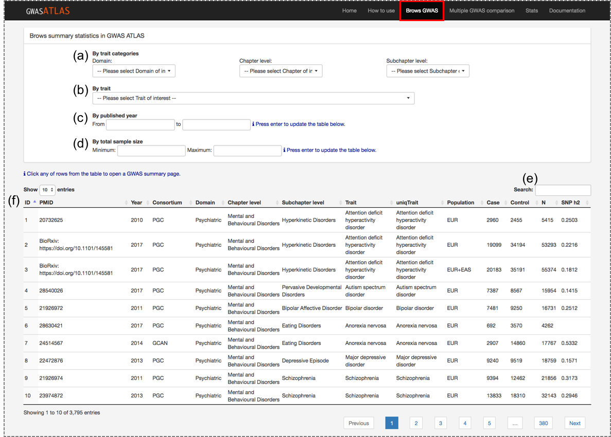
Go to the "Browse GWAS" page which displays a table of entire entries of GWAS summary statistics in the database.
If you know which trait you are looking for, you can either select from the list of traits (b)
or type the trait name in the search box (e).
If you are just looking for what kind of traits are available in the database,
you can also filter by domain, chapter or subchapter level (a).
Traits can also be filtered by published year and sample size in the filtering boxes (c and d).
Any key ward can be searched from the search box (e).
Each GWAS in the table (f) is clickable which will open a new tab with detailed information.
(a) Filtering by trait categories.
(b) Select by trait name.
(c) Filtering by published year.
(d) Filtering by total sample size.
(e) Search box.
(f) GWAS entries.
(a) Filtering by trait categories.
(b) Select by trait name.
(c) Filtering by published year.
(d) Filtering by total sample size.
(e) Search box.
(f) GWAS entries.
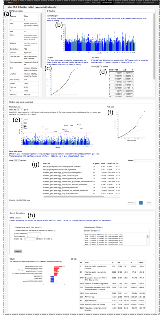
1.2. Summary of GWAS results (right image)
When a GWAS is clicked, it will open a new tab with summary of the following results results.(a) GWAS information table: There are variety of basic information about the study. Original study is accessible from PMID field. Original summary statistics file can be accessed from the link. Details of each feature is available in 3. Database features in the documentation. (b) Manhattan plot
(c) Q-Q plot
(d) List of top SNPs in each genomic risk locus
(e) Gene manhattan plot: P-value is based on MAGMA gene ananlysis. Top genes can be labeled by changing the number of the box.
(f) Gene Q-Q plot
(g) Top associated gene set: Results of MAGMA gene-set analysis. Gene sets which are significantly associated after Bonferroni correction are displayed. If the number of significant gene sets are less than 10, top 10 significant gene sets are displayed.
(h) Generic correlation: Genetic correlation of the selected trait with other traits in the database. See next section for details.
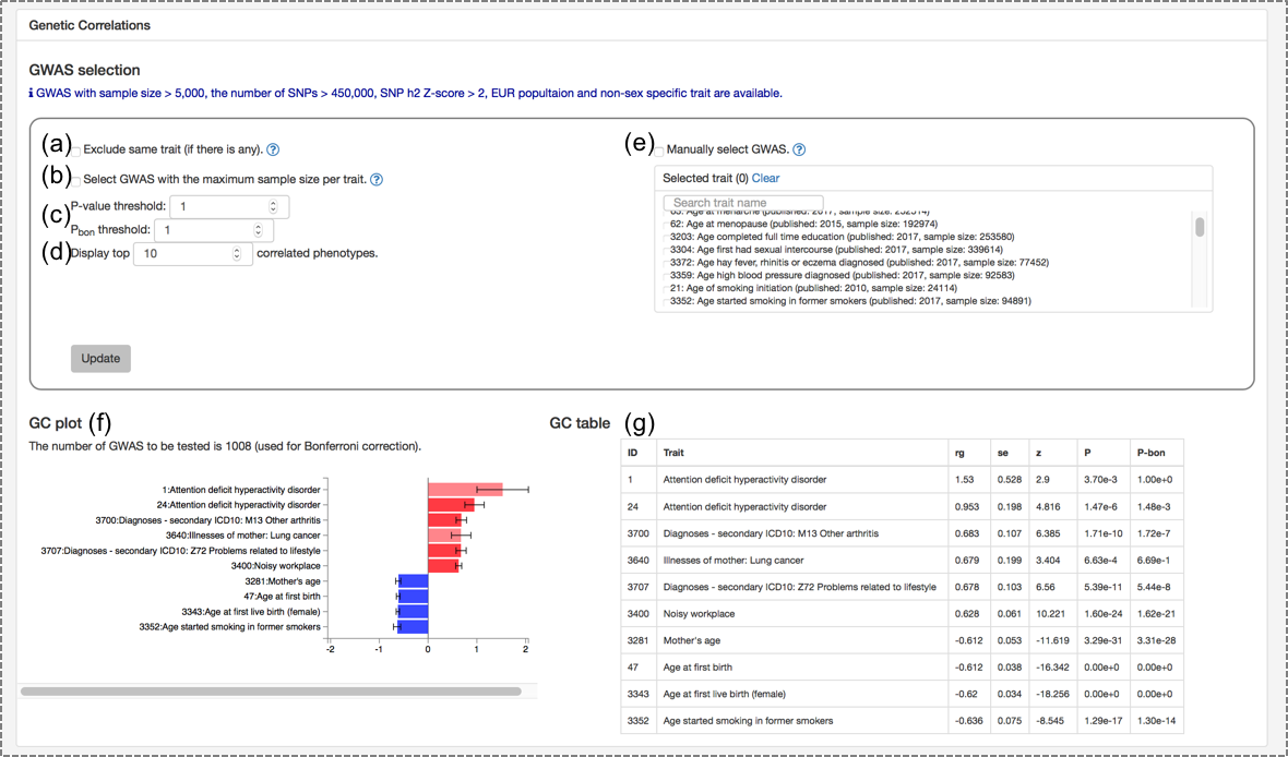
1.3. Genetic correlation (bottom image)
By default, top 10 traits with the highest absolute genetic correlation are displayed regardless of significance. Nothing is shown for traits which are not eligible for estimation of genetic correlation (see 5.3. Genetic correlation in the Documentation). Several options are available to obtain genetic correlation with a custom list of traits as the followings.(a) Exclude the same trait: If there is any other traits with the same name in the "uniqTrait" feature in the database, those can be excluded by activating this option.
(b) Select GWAS with the maximum sample size per trait: For traits with more than one GWAS in the database, one with the largest sample size is selected per trait. Note that this selection is performed after other filtering options.
(c) P-value and Bonferroni corrected P-value threshold.
(d) The number of traits to display. (e) Manual selection of trait: Traits can also be manually selected. Other filtering options are still performed on the selected traits.
(f) Genetic correlation plot: Each bar is colored based on P-value; grey for P-value >= 0.05, high transparency red (positive) and blue (negative) for P-value < 0.05, and red or blue for P-value < Pbon. Bonferroni correction is performed for the number of possible pairs before filtering of P-value but after other filtering options.
(g) Genetic correlation table: same as (f) but in table format.
2. Compare multiple GWAS
2.1. Select GWAS to compare
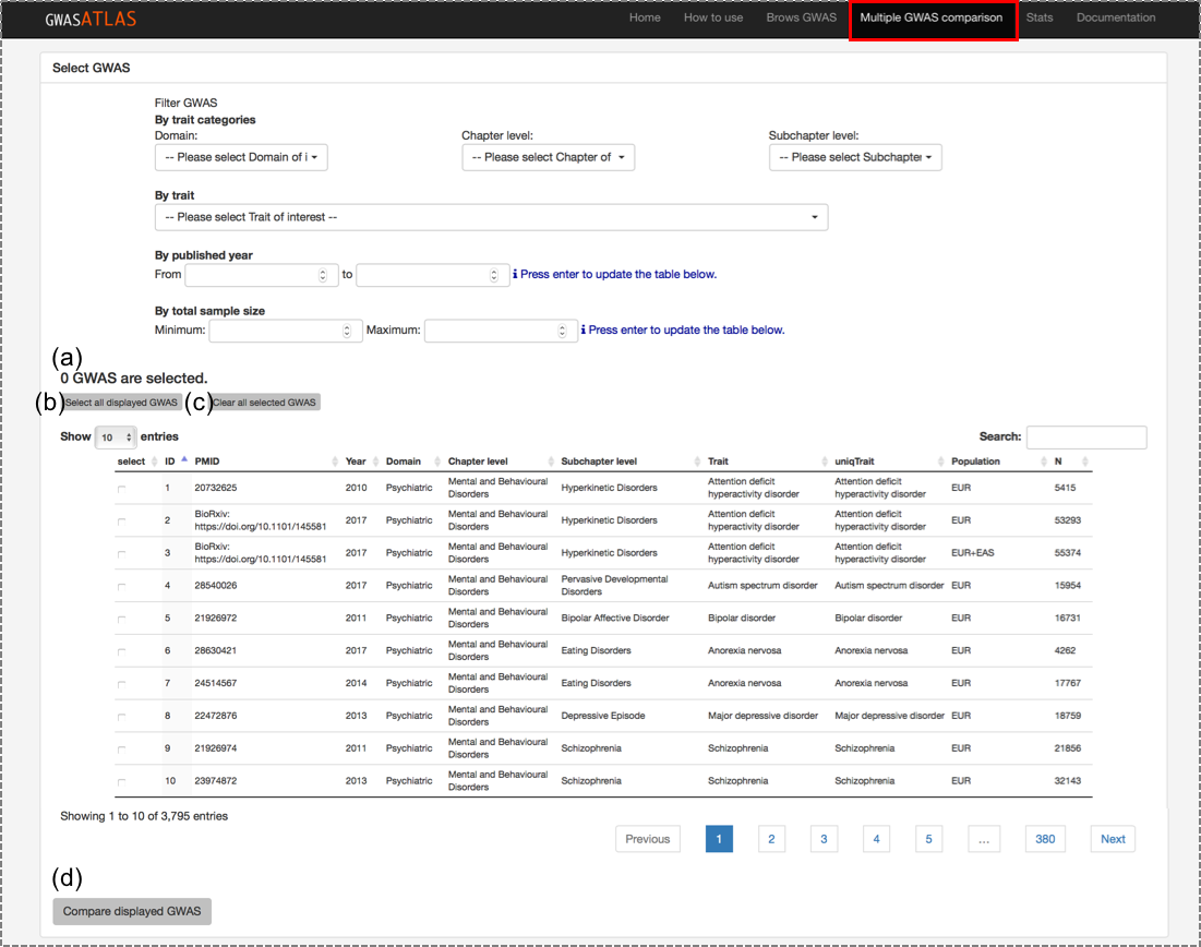
Go to "Multiple GWAS comparison" page.
Database entries can be filtered same as in the "Browse GWAS" page.
GWAS can be selected by checking the box manually or using buttons described below.
(a) Number of selected GWAS: This number should be > 1 and ≤ 100.
(b) Select all displayed GWAS: this button only checks "currently displayed" GWAS, but not all the GWAS after filtering. You can change the number of GWAS to display from the left top of the table.
(c) Clear all selected GWAS: Reset the selection of GWAS regardless of displayed or not.
(d) Submit selected GWAS
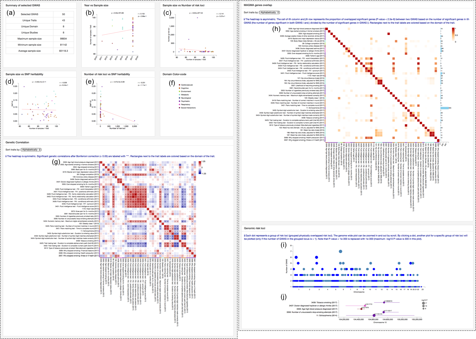
2.2. Summary of results
When selected GWAS are submitted correctly, several plots will be displayed in the page. See 7. Multi GWAS comparison of documentation for details.(a) Summary of selected GWAS.
(b) Scatterplot of published year and sample size: Each dot is a GWAS colored by domain.
(c) Scatterplot of sample size and number of risk loci: Each dot is a GWAS colored by domain.
(d) Scatterplot of SNP heritability and sample size: Each dot is a GWAS colored by domain.
(e) Scatterplot of SNP heritability and number of risk loci: Each dot is a GWAS colored by domain.
(f) Color code: Color of each domain. This color code is used in all plots in the page.
(g) Genetic correlation heatmap: Each cell is colored by rg and sized by P-value. The significant ones are labeled by "*". The order of row and column can be selected from alphabetically, domain and hierarchical clustering. The color of rectangles next to the GWAS label represent the color of domain.
(h) MAGMA gene overlap heatmap: Each cell is colored by proportion of overlapping significant genes. The order of row and column can be selected from alphabetically, domain and hierarchical clustering. The color of rectangles next to the GWAS label represent the color of domain.
(i) Manhattan like plot of risk loci: Each dot is a locai group (see 7.4. Risk loci overlap in the documentation for details) sized by the the number of GWAS in the loci group (same as Y-axis). The plot is zoomable and it will display plot (j) by cliking a dot.
(j) Zoomed plot of a selected loci group: Each dot represents a top SNP in the locus of given GWAS sized by P-value, colored by domain and labelled by rsID. A horizontal line represents the region of the risk locus. See 4.2. Risk loci in the documentation for the definition of risk loci.
